Matrix Multiplication

Table of Contents

• Problem Formulation
• Parallel Patterns
• Benchmarking

We study the classic problem, 2D matrix multiplication. We will start with a short introduction about the problem and then discuss how to solve it parallel CPUs.

Problem Formulation

We are multiplying two matrices, A (MxK) and B (KxN). The numbers of columns of A must match the number of rows of B. The output matrix C has the shape of (MxN) where M is the rows of A and N the columns of B. The following example multiplies a 3x3 matrix with a 3x2 matrix to derive a 3x2 matrix.

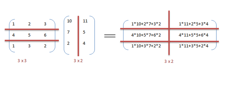
As a general view, for each element of C we iterate a complete row of A and a complete column of B, multiplying each element and summing them.

We can implement matrix multiplication using three nested loops.

for(int m=0; m<M; m++) {
  for(int n=0; n<N; n++) {
    C[m][n] = 0;
    for(int k=0; k<K; k++) {
      C[m][n] += A[m][k] * B[k][n];
    }
  }
}

Parallel Patterns

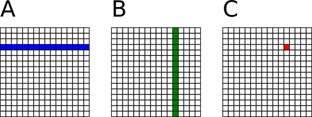
At a fine-grained level, computing each element of C is independent of each other. Similarly, computing each row of C or each column of C is also independent of one another. With task parallelism, we prefer coarse-grained model to have each task perform rather large computation to amortize the overhead of creating and scheduling tasks. In this case, we avoid intensive tasks each working on only a single element. by creating a task per row of C to multiply a row of A by every column of B.

// C = A * B
// A is a MxK matrix, B is a KxN matrix, and C is a MxN matrix
void matrix_multiplication(int** A, int** B, int** C, int M, int K, int N) {
  tf::Taskflow taskflow;
  tf::Executor executor;
  for(int m=0; m<M; ++m) {
    taskflow.emplace([m, &] () {
      for(int n=0; n<N; n++) {
        for(int k=0; k<K; k++) {
          C[m][n] += A[m][k] * B[k][n];  // inner product
        }
      }
    });
  }
  executor.run(taskflow).wait();
}

Instead of creating tasks one-by-one over a loop, you can leverage Taskflow::for_each_index to create a parallel-for task. A parallel-for task spawns a subflow to perform parallel iterations over the given range.

// perform parallel iterations on the range [0, M) with the step size of 1
tf::Task task = taskflow.for_each_index(0, M, 1, [&] (int m) {
  for(int n=0; n<N; n++) {
    for(int k=0; k<K; k++) {
      C[m][n] += A[m][k] * B[k][n];
    }   
  }   
}); 

Please visit Parallel Iterations for more details.

Benchmarking

Based on the discussion above, we compare the runtime of computing various matrix sizes of A, B, and C between a sequential CPU and parallel CPUs on a machine of 12 Intel i7-8700 CPUs at 3.2 GHz.

A	B	C	CPU Sequential	CPU Parallel
10x10	10x10	10x10	0.142 ms	0.414 ms
100x100	100x100	100x100	1.641 ms	0.733 ms
1000x1000	1000x1000	1000x1000	1532 ms	504 ms
2000x2000	2000x2000	2000x2000	25688 ms	4387 ms
3000x3000	3000x3000	3000x3000	104838 ms	16170 ms
4000x4000	4000x4000	4000x4000	250133 ms	39646 ms

The speed-up of parallel execution becomes clean as we increase the problem size. For example, at 4000x4000, the parallel runtime is 6.3 times faster than the sequential runtime.